Do you know that you can utilize Google Sheets’ VLOOKUP function with multiple criteria?
Suppose you wish to utilize the Vlookup function to find a value based on the first and last name.
This post will explain how to Vlookup multiple criteria in Google Sheets using various scenarios.
1. Vlookup Multiple Criteria into Single Column
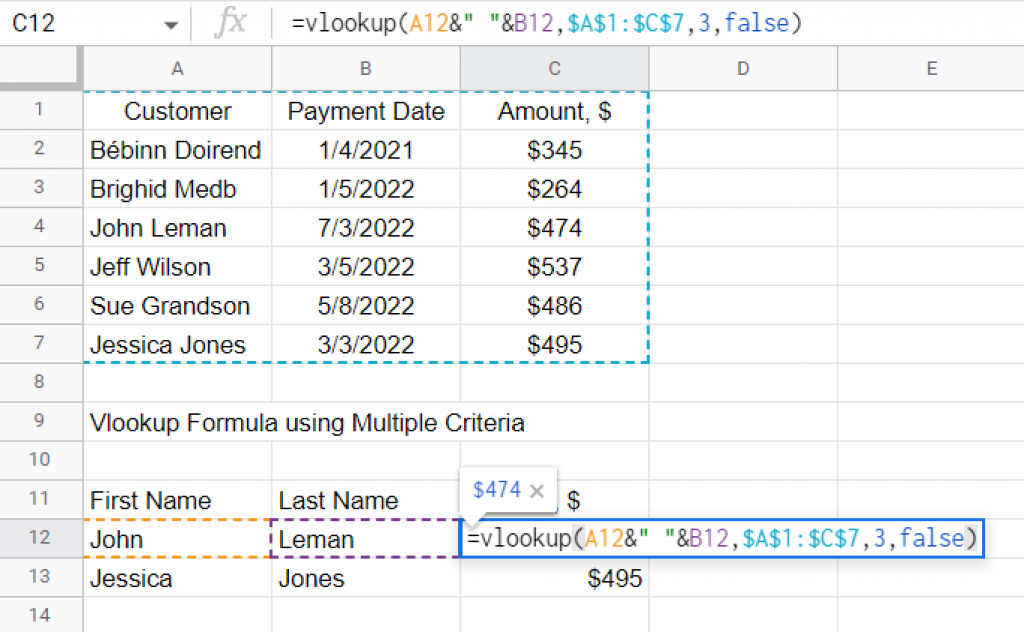
In the following example, we search the full table for first and last names (from two separate cells). If an exact match is found, the amount specified in the last column is shown.
Assume we wish to combine search criteria for the Vlookup formula. Let’s say we know a person’s first and last name, but the table we wish to search only contains a combined full name column.
In order to combine the criteria before searching, the technique in this case is to nest a concatenation formula within the Vlookup.
The formula for this Vlookup with multiple criteria in Google Sheets is fairly simple:
=VLOOKUP(A15&" "&B15,$A$1:$C$9,3,false)

where:
- A12&” “&B12 = concatenates the first name and last name from A12 and B12
- $A$1:$C$7 = the range table in which to search
- 3 = the column number we wish to display if a match is discovered
This is a standard Vlookup formula with the first argument consisting concatenated values. Before looking for the entire name in the table, we must first merge the first and last names.
The first parameter of the formula displayed concatenates the first and last name, and this value is then searched inside the table using the Vlookup function.
2. Vlookup Single Criteria into Multiple Columns
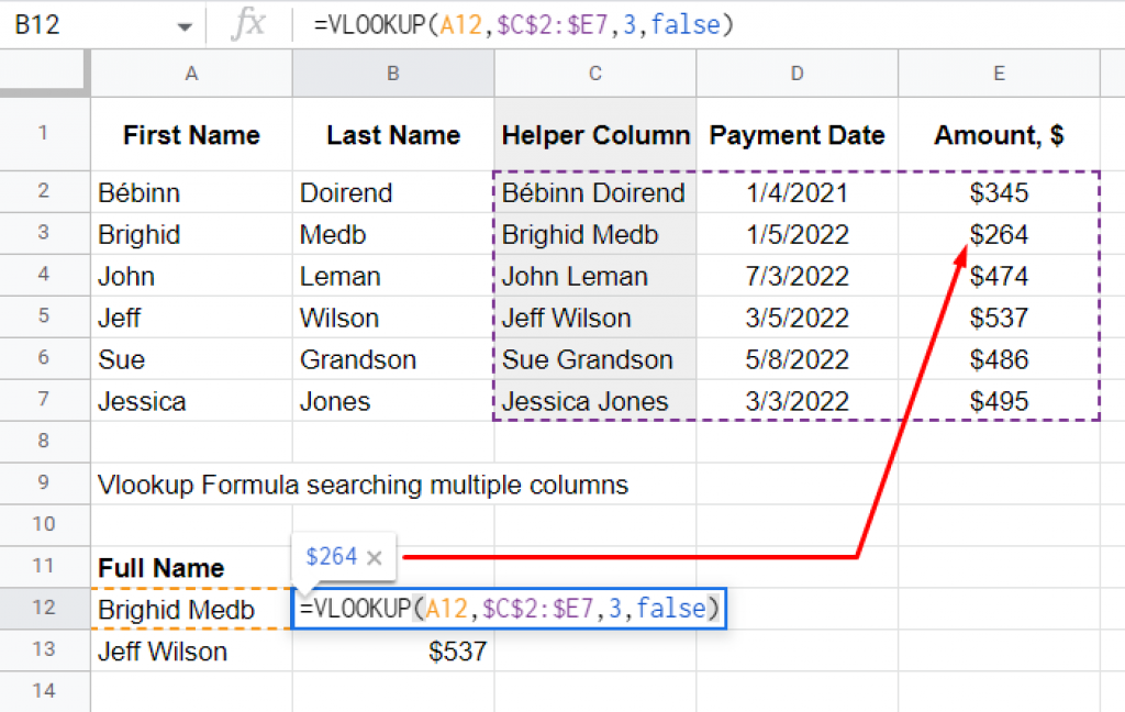
This scenario is the opposite of the previous one. So, while we have a full search phrase, our search table has numerous columns that must be searched.
For instance, the search table contains a column for first name and a column for last name, despite the fact that our search query is someone’s whole name. We can’t use a conventional vlookup in this case.
We concantenate the necessary cells into a new search column by creating a helper column in the search table. As a result, we merge the first and last names in order to generate a helper column with the full name.
=VLOOKUP(A12,$C$2:$E7,3,false)

We can use any of the following formulas in order to concatenate in Google Sheets, in our example, first name and last name:
=A1&” “&B1
=CONCATENATE(A1,” “,B1)
=JOIN(” “,A1:B1)
3. Vlookup Single Criteria into Multiple Columns with Array Formulas
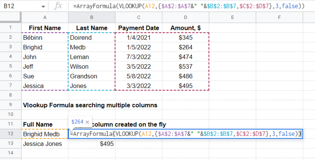
In this situation, we perform the same thing as in the prior scenario, but the difference is that this helper column is created dynamically on the fly rather than in the table. As a result, we shall utilize an Array Formula.
=ArrayFormula(VLOOKUP(A12,{$A$2:$A$7&” “&$B$2:$B$7,$C$2:$D$7},3,false))

In order to break down this formula, we have to a) create an array of criteria columns and b) add the other columns from the original table.
a) Create the array of criteria columns. To begin, use the following formula to create an array of full names:
=ArrayFormula(A12,{$A$2:$A$7&” “&$B$2:$B$7)
After you’ve entered this formula, use Ctrl + Shift + Enter (Windows) or Cmd + Shift + Enter (Mac) to add the Array Formula designation.
The end result is that the whole names are retrieved.
b) Add the other columns from the initial table. In this stage, we create a new search table by adding the other columns from the original table that we wish to search for, using the following formula:
=ArrayFormula({$A$2:$A$7&” “&$B$2:$B$7,$C$2:$D$7})
In this stage, we receive the first and last name in one column, as well as two extra columns from the range table: Payment Date and Amount.
In the end, we may perform the vlookup. So we made a new table with the full name column and used it as the range input in a typical vlookup using the following formula:
=ArrayFormula(VLOOKUP(A12,{$A$2:$A$7&” “&$B$2:$B$7,$C$2:$D$7},3,false))


